kaepora is an open-source relational database for Type Ia Supernova spectra. For installation and example code please visit our Read the Docs page. You can download the source code from our Github repository Below are links to download the most recent versions of the database:

After downloading, unzip and place the ‘.db’ file in the /data folder of the repository.

I am currently the only active developer regarding database architecture and user interaction. If you would like to contribute, please contact me and I will add you as a github collaborator. Let me know if you have suggestions for how I can improve this tool. If you have metadata that you think would be interesting to include, I am happy to help.

Can Measuring SN Ia Velocities Improve Cosmological Distance Measurements?

We used kaepora to investigate the spectra of 126 SNe Ia that have cosmological distance measurements. Using composite spectra, we found evidence that SNe with negative Hubble Residuals (those with underestimated distances relative to a cosmological model) tend to have higher velocities. In the figure to the right, we show the velocity evloution of the Si II $\lambda$6355 feature for the positive/negative (blue/red) Hubble Residual samples. For more information please take a look at our recent paper (Siebert et al. 2020)

Composite Spectra

Below are the composite spectra presented in Siebert et al. 2019. All of these have been constructed using our “Gini-Weighting” method that is described in the paper.

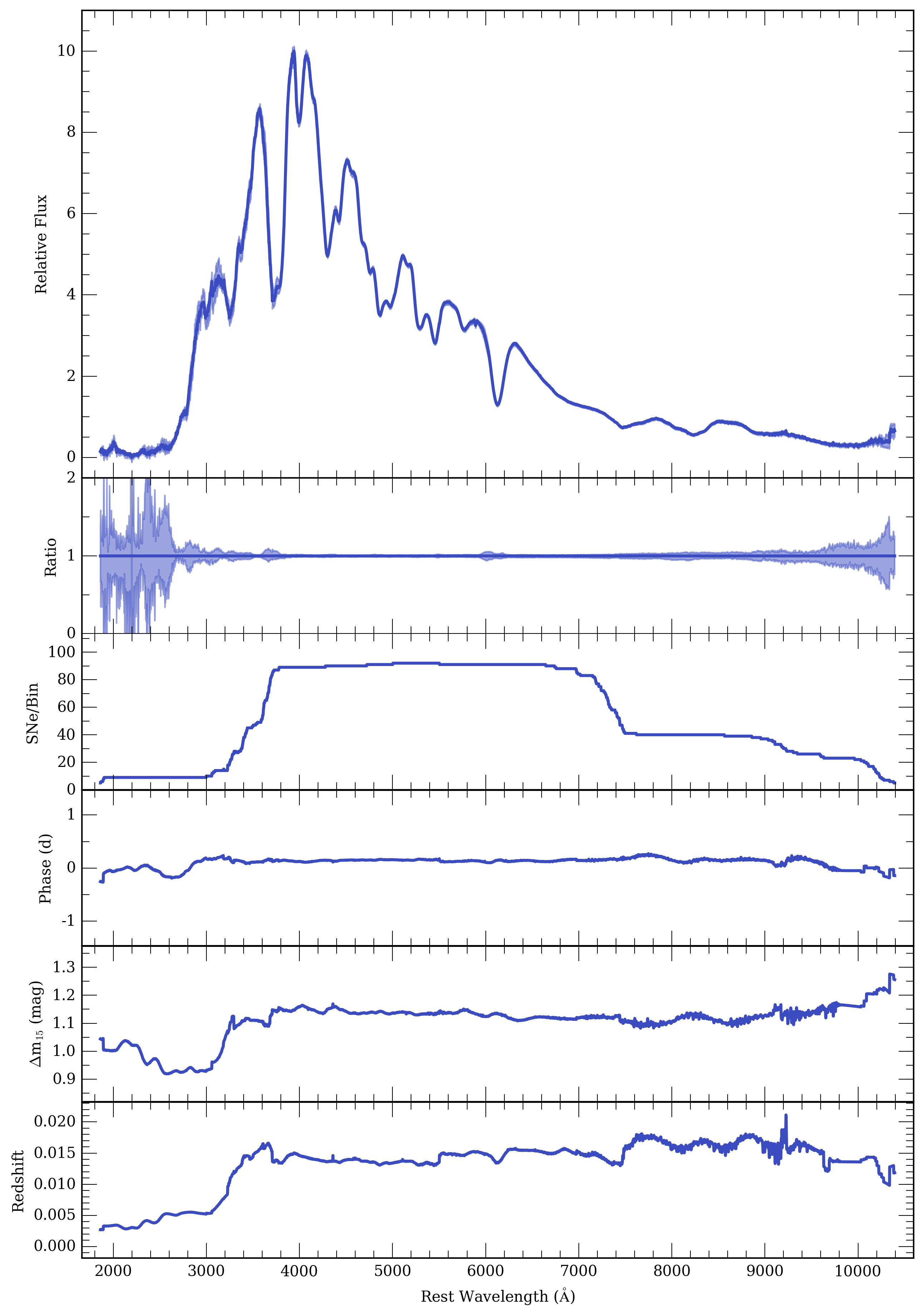
Each spectrum contains 7 columns of data. They are wavelength (A), flux (arbitrary), $1\sigma$ lower bootstrap sampling error (arbitrary), $1\sigma$ upper bootstrap sampling error (arbitrary), phase (rest-frame days), $\Delta m_{15}$ $(B)$ (mag), redshift, and the number of SNe per wavelength bin. At the top of each file we also include the SQL query that was used to generate the composite spectrum. Follow the link below to view the example composite spectrum from Figure 14 (right) in our paper.

siebert_example_max_light

Sets of Composite Spectra from Siebert et al. 2019

All Composite Spectra	siebert_all.tar
Phase-Binned	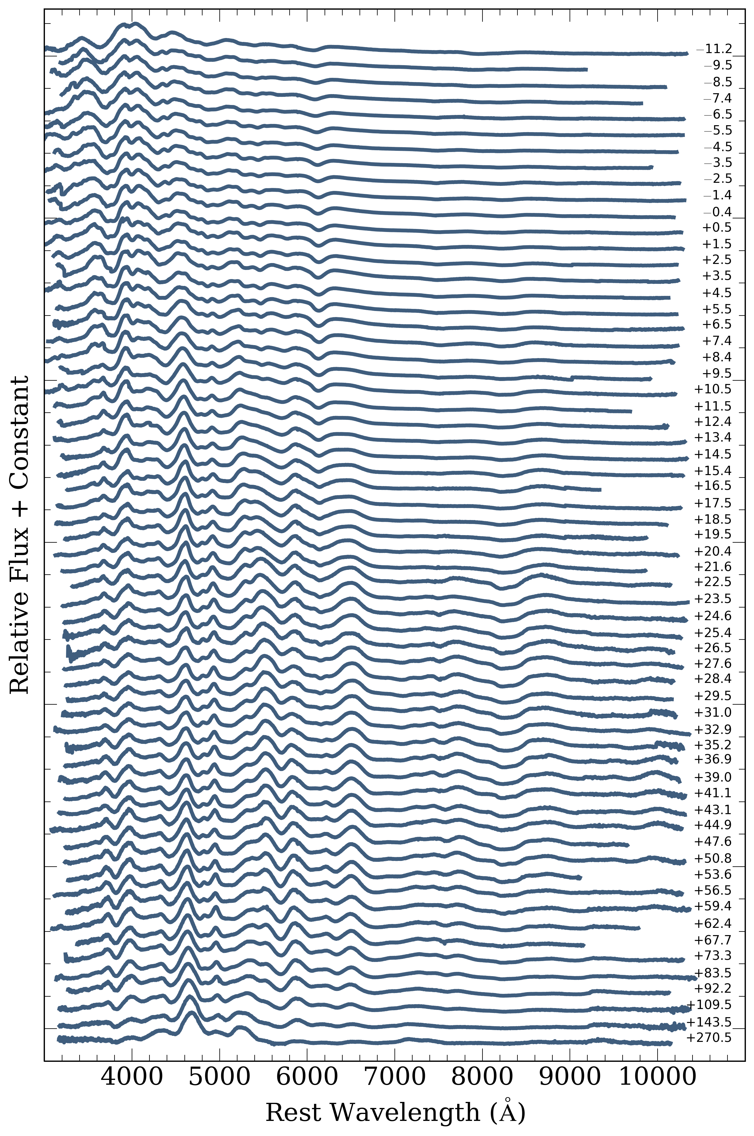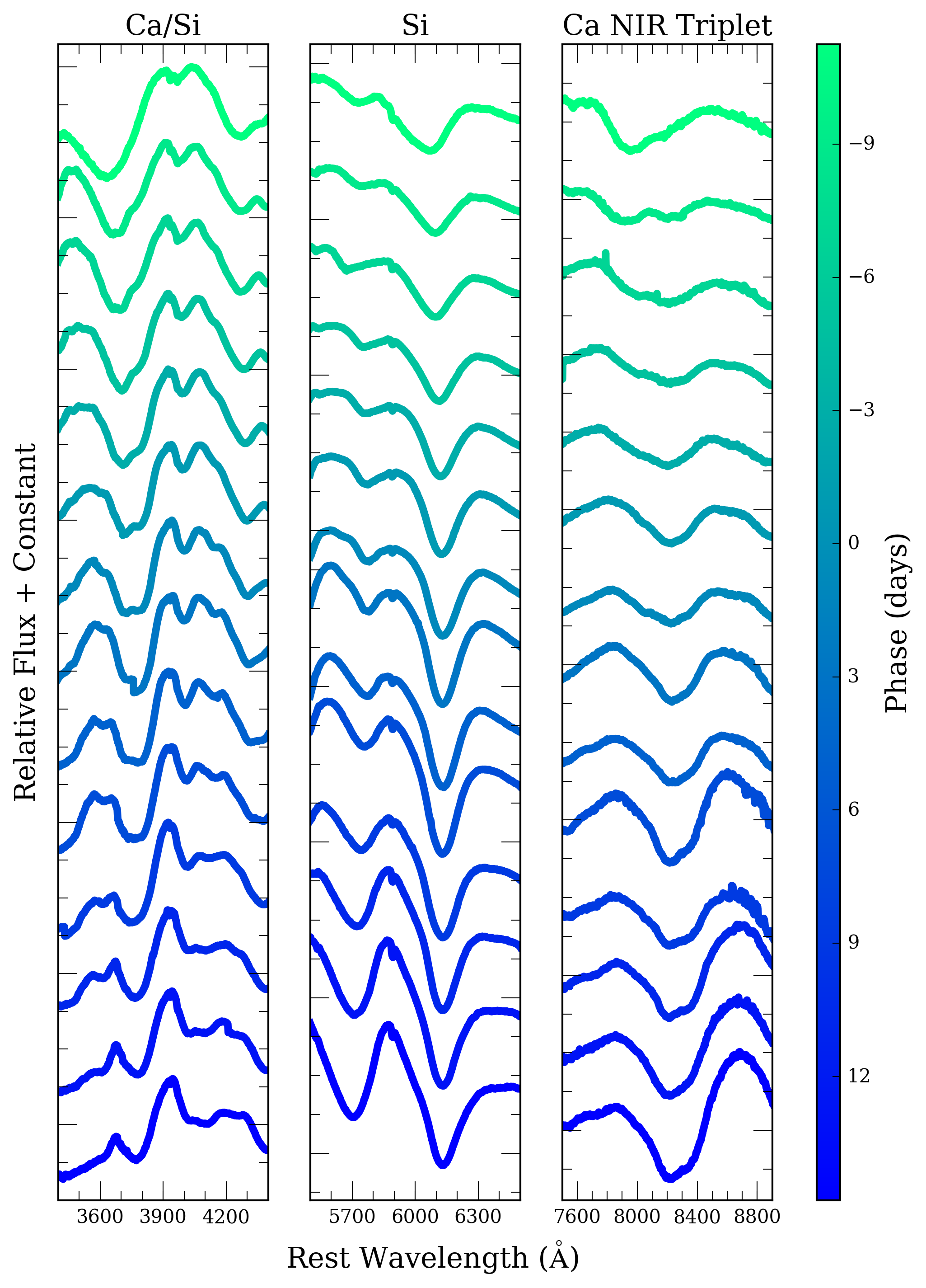siebert_phase.tar siebert_phase_2day.tar
Color Curve	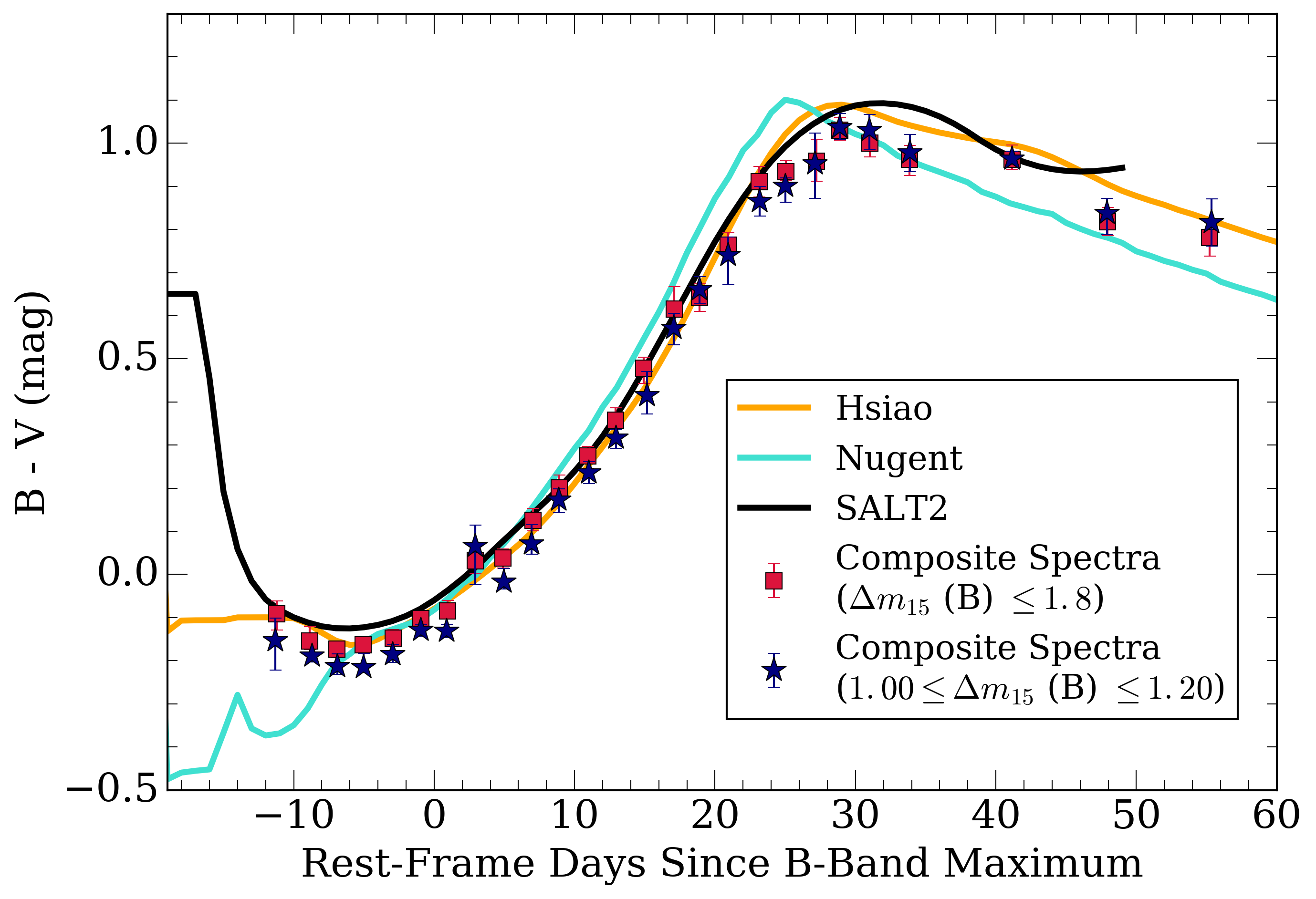siebert_color_curve.tar
Maximum-Light $\Delta m_{15}$ $(B)$-Binned	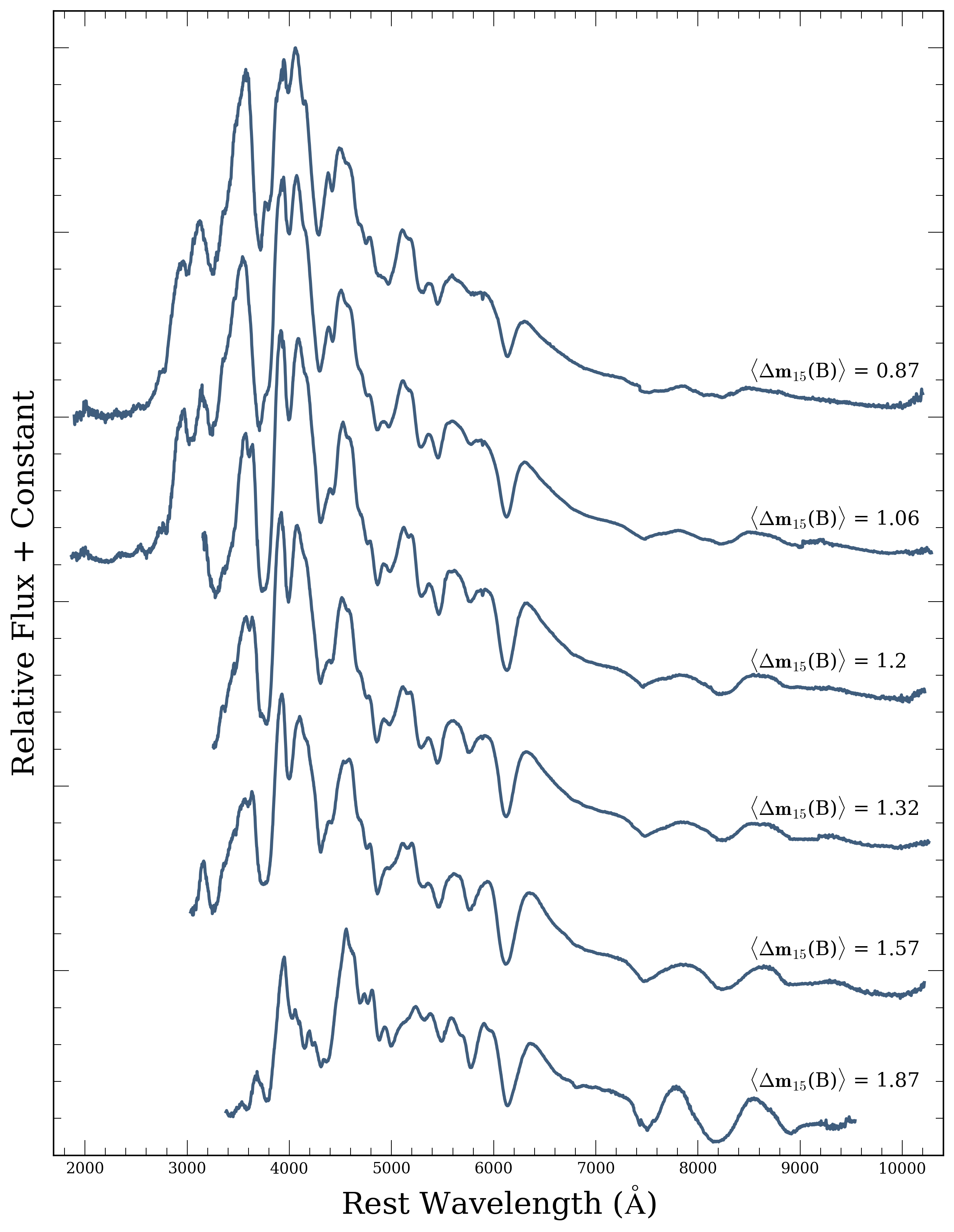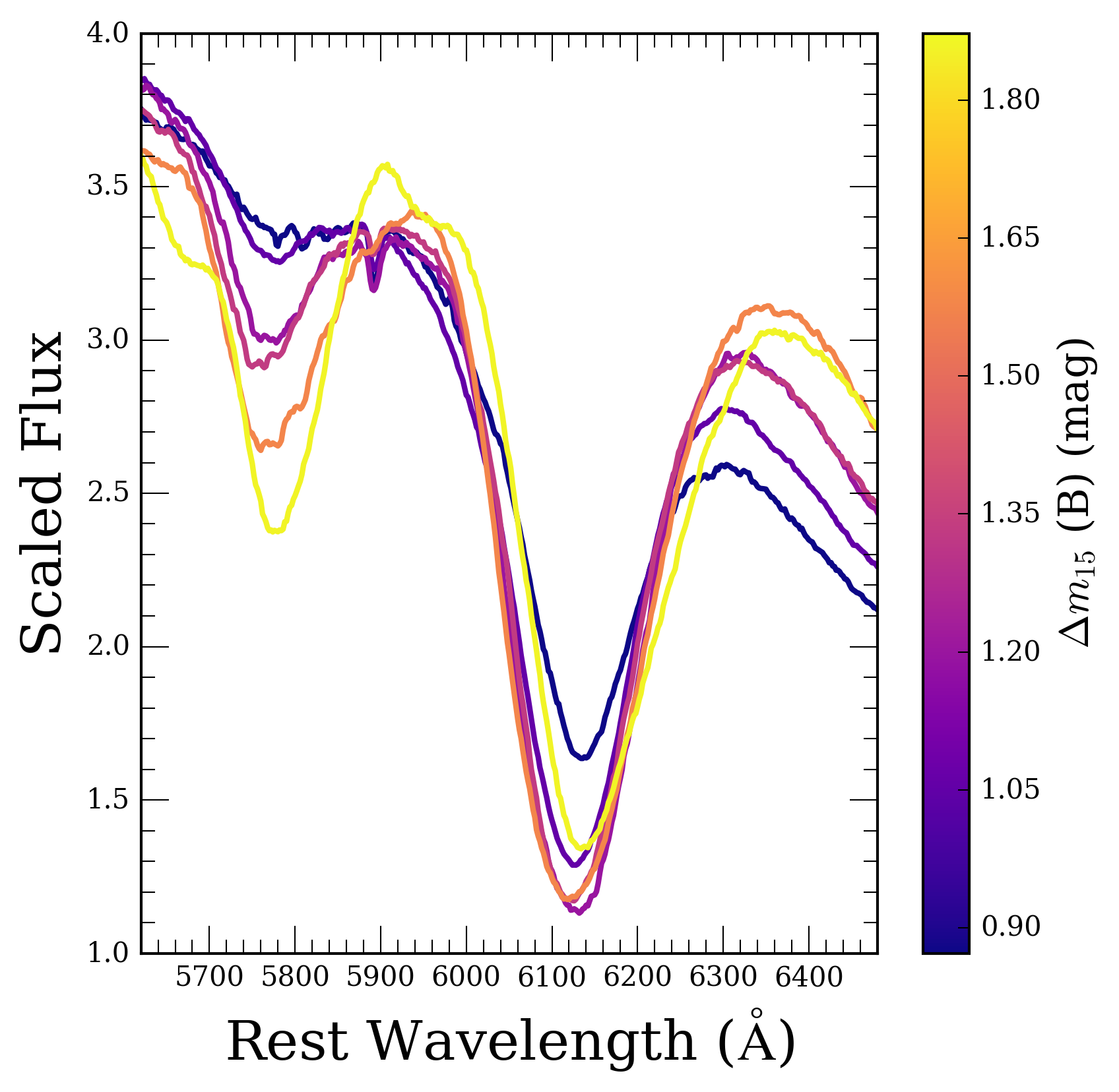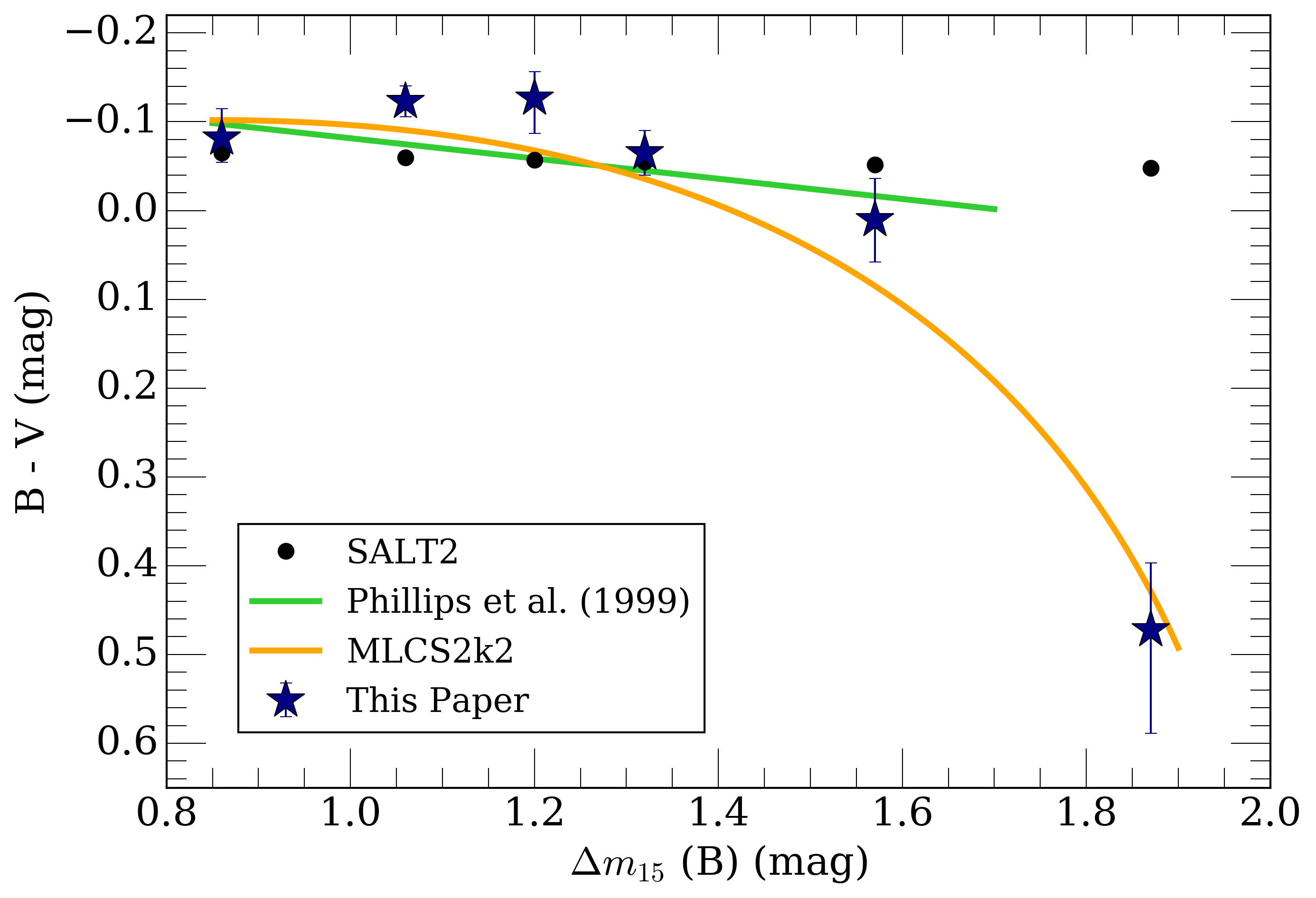siebert_max_light_dm15.tar
Phase-$\Delta m_{15}$ $(B)$ Grid	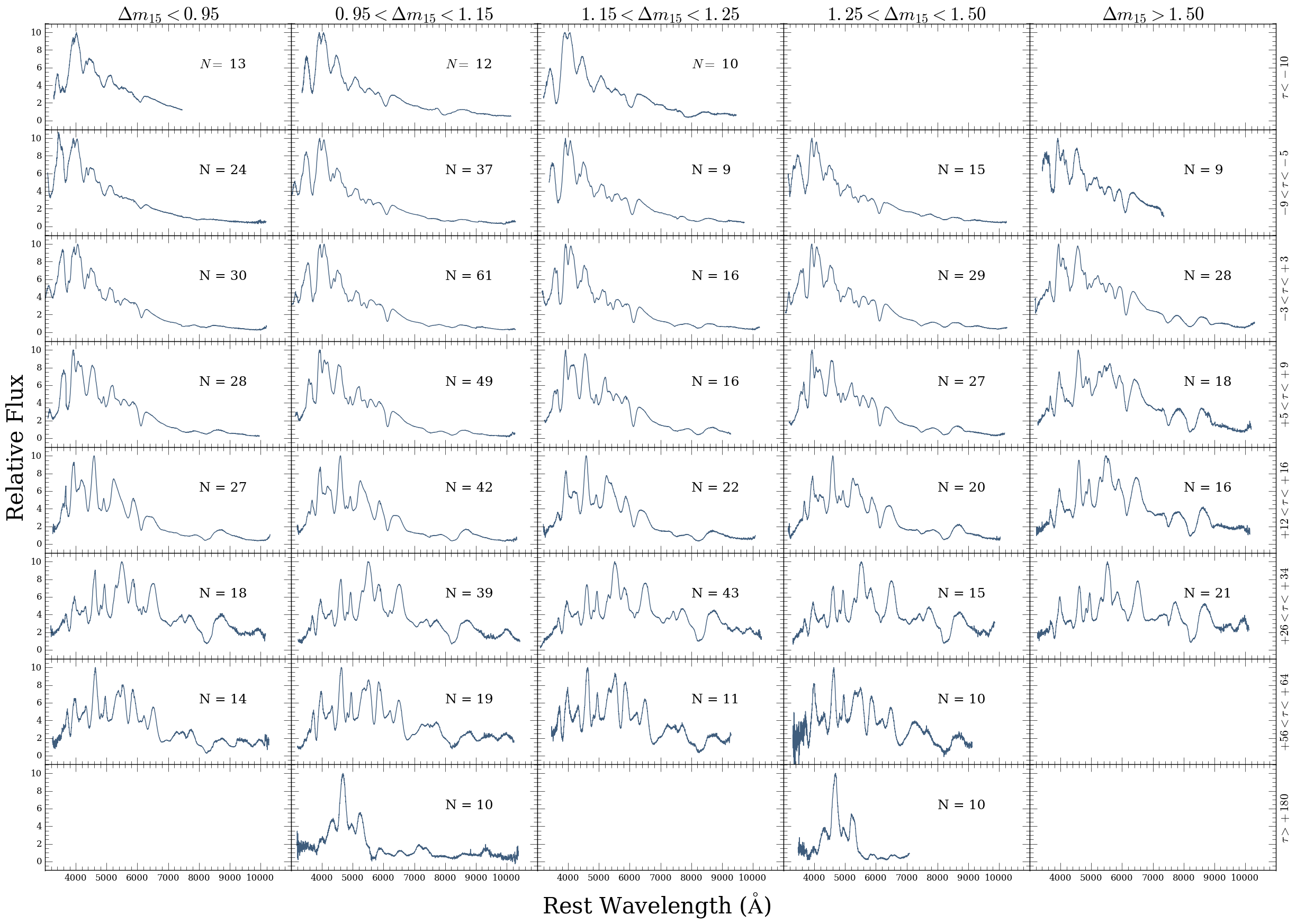siebert_grid.tar
Template Comparisons	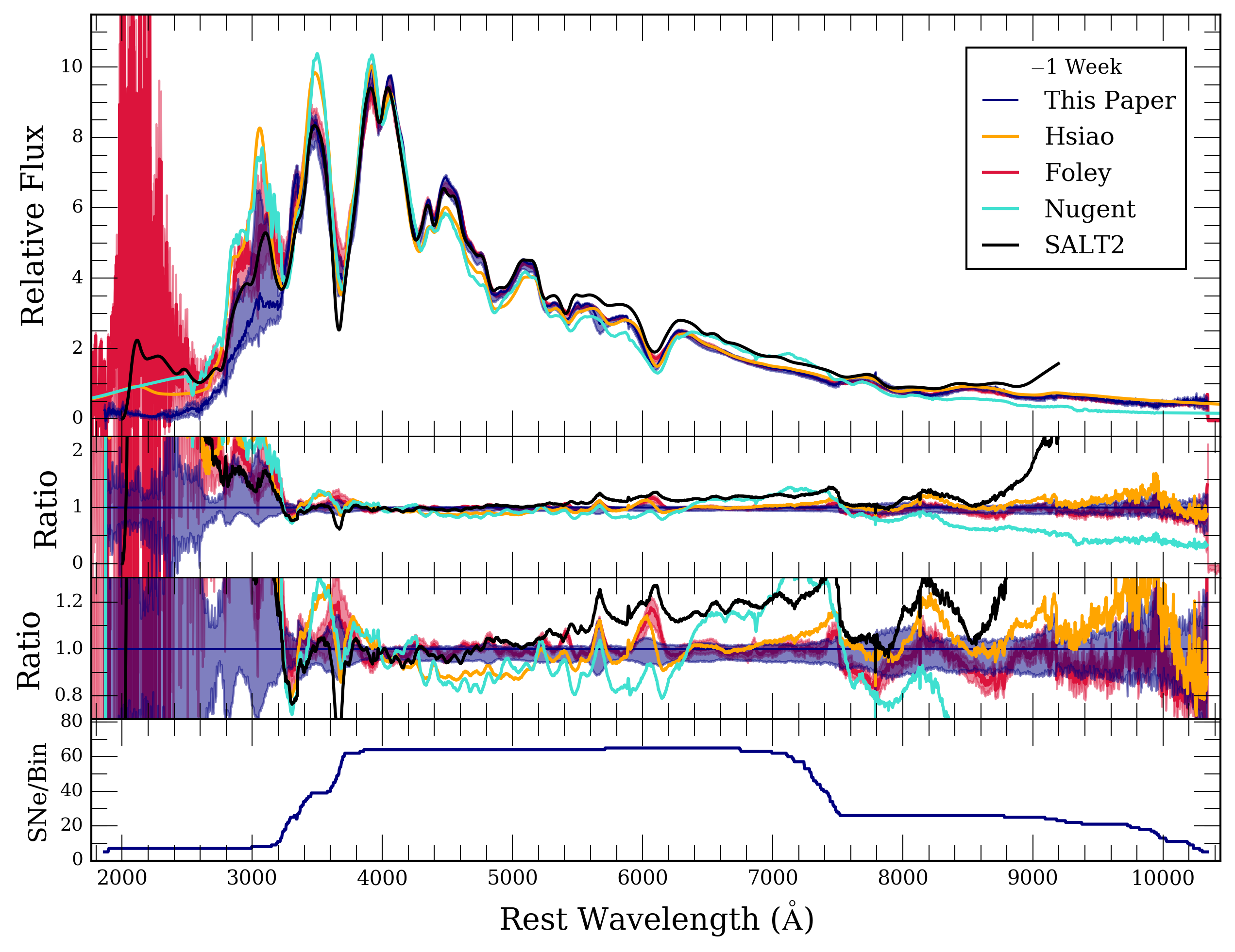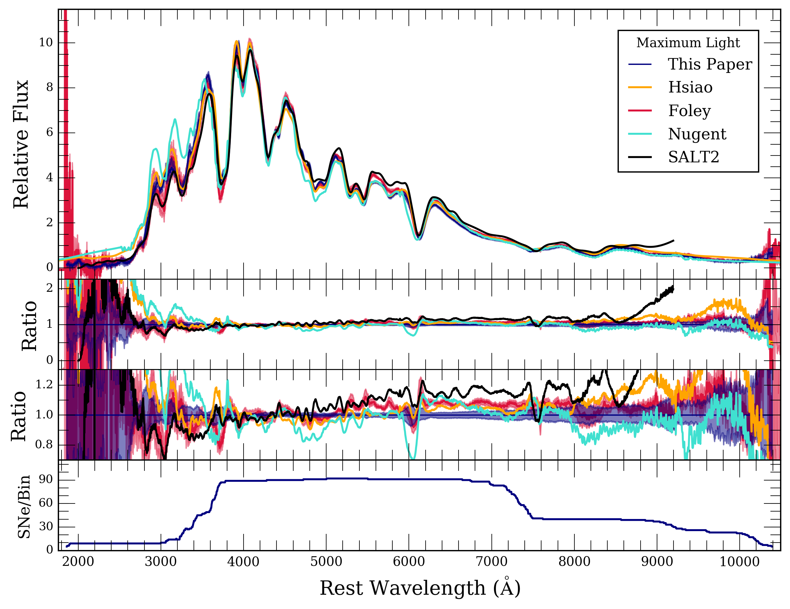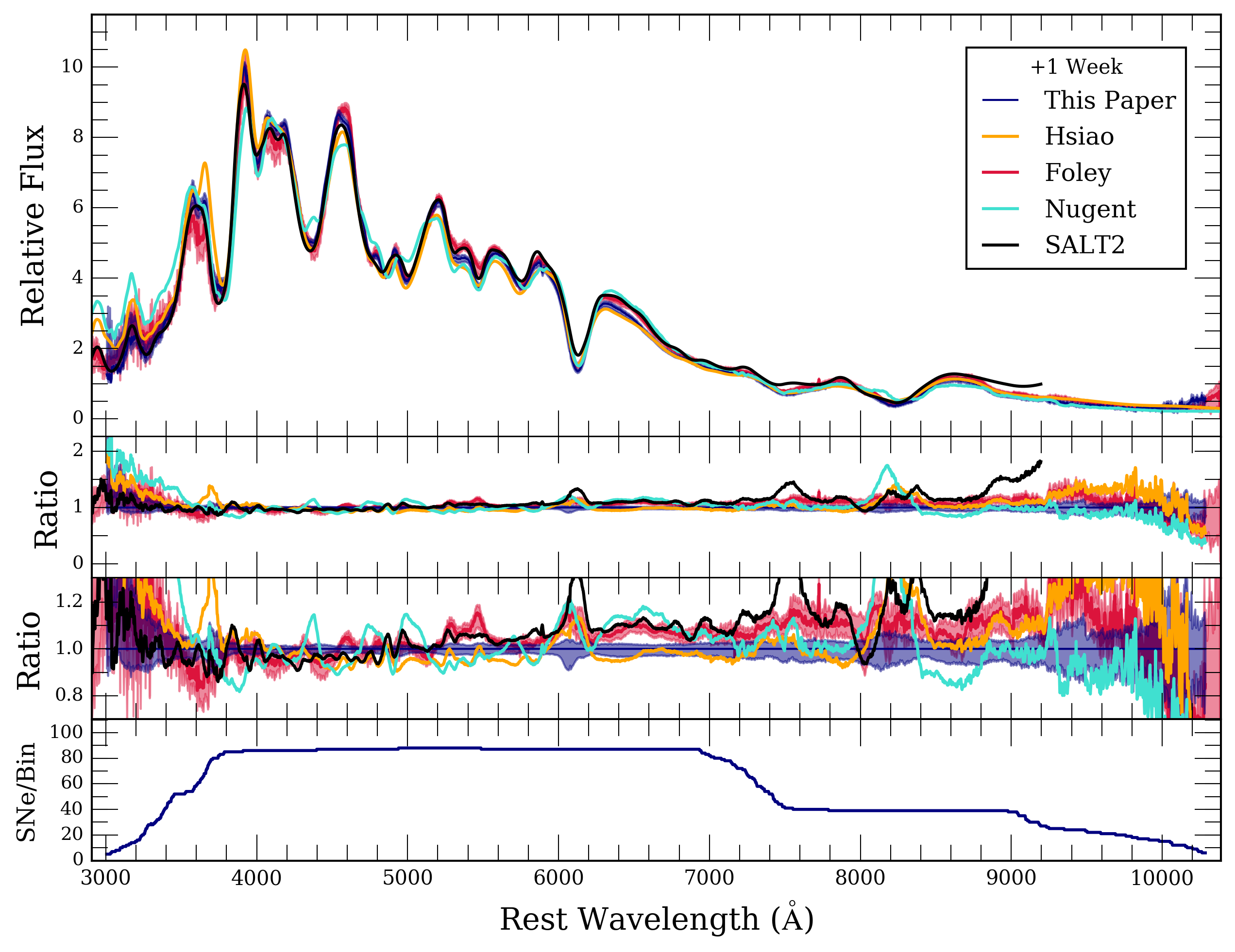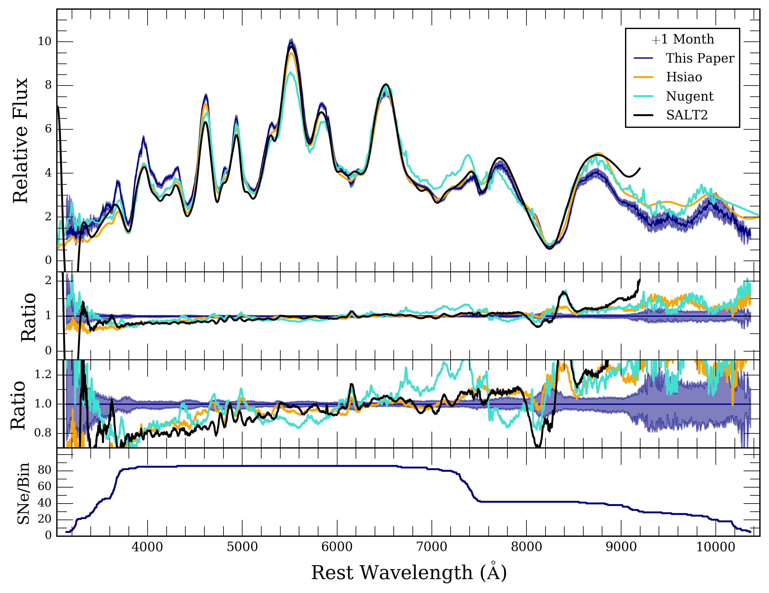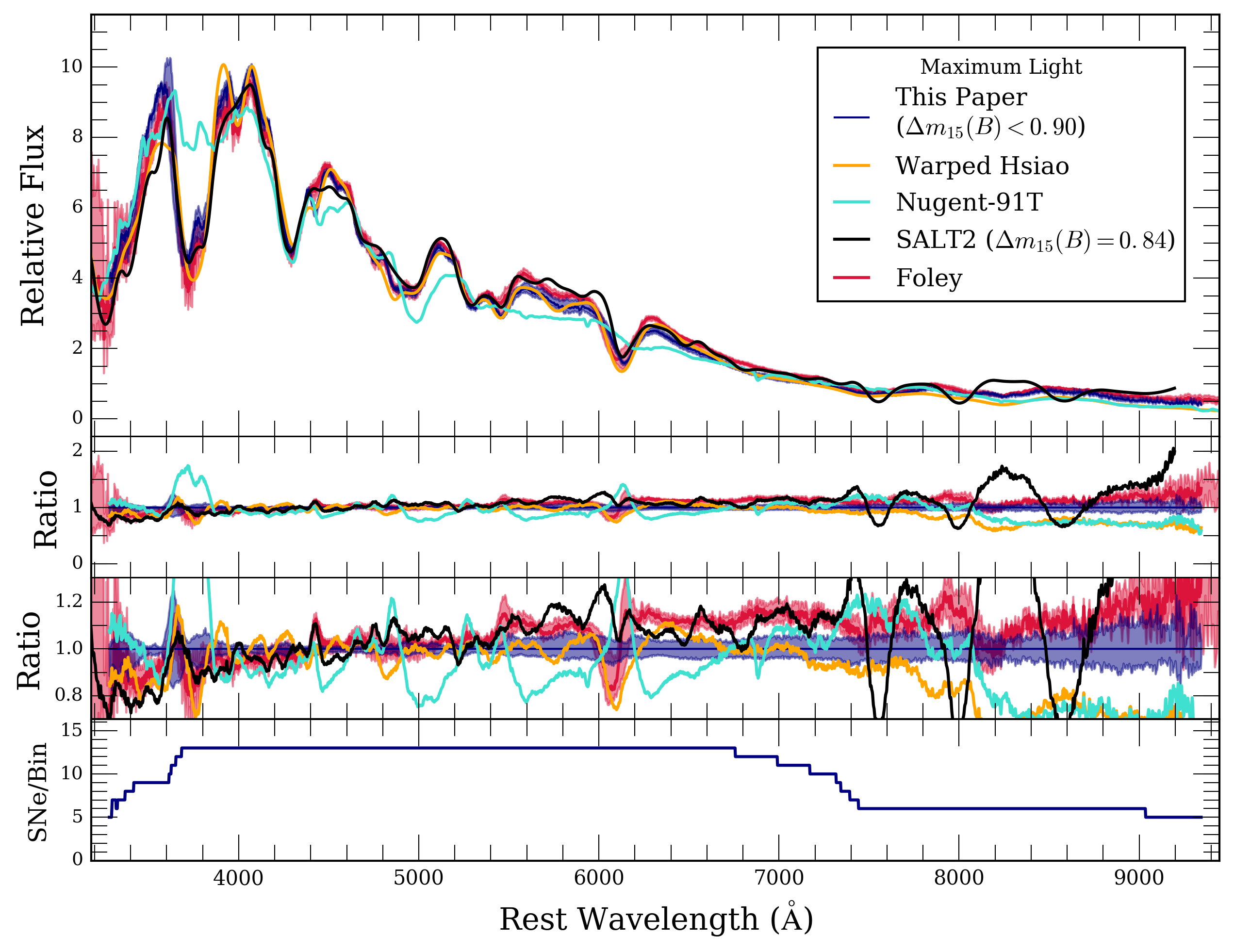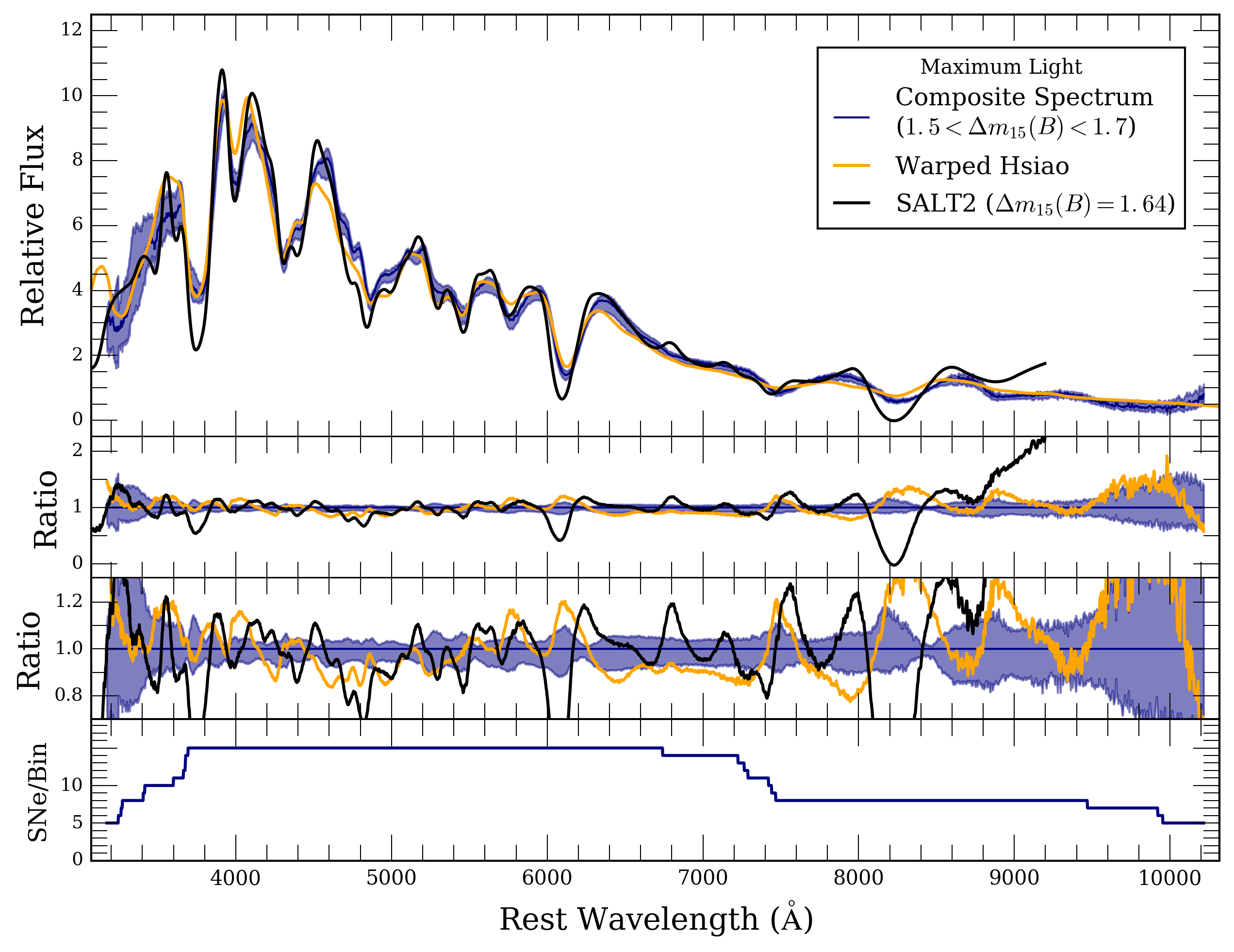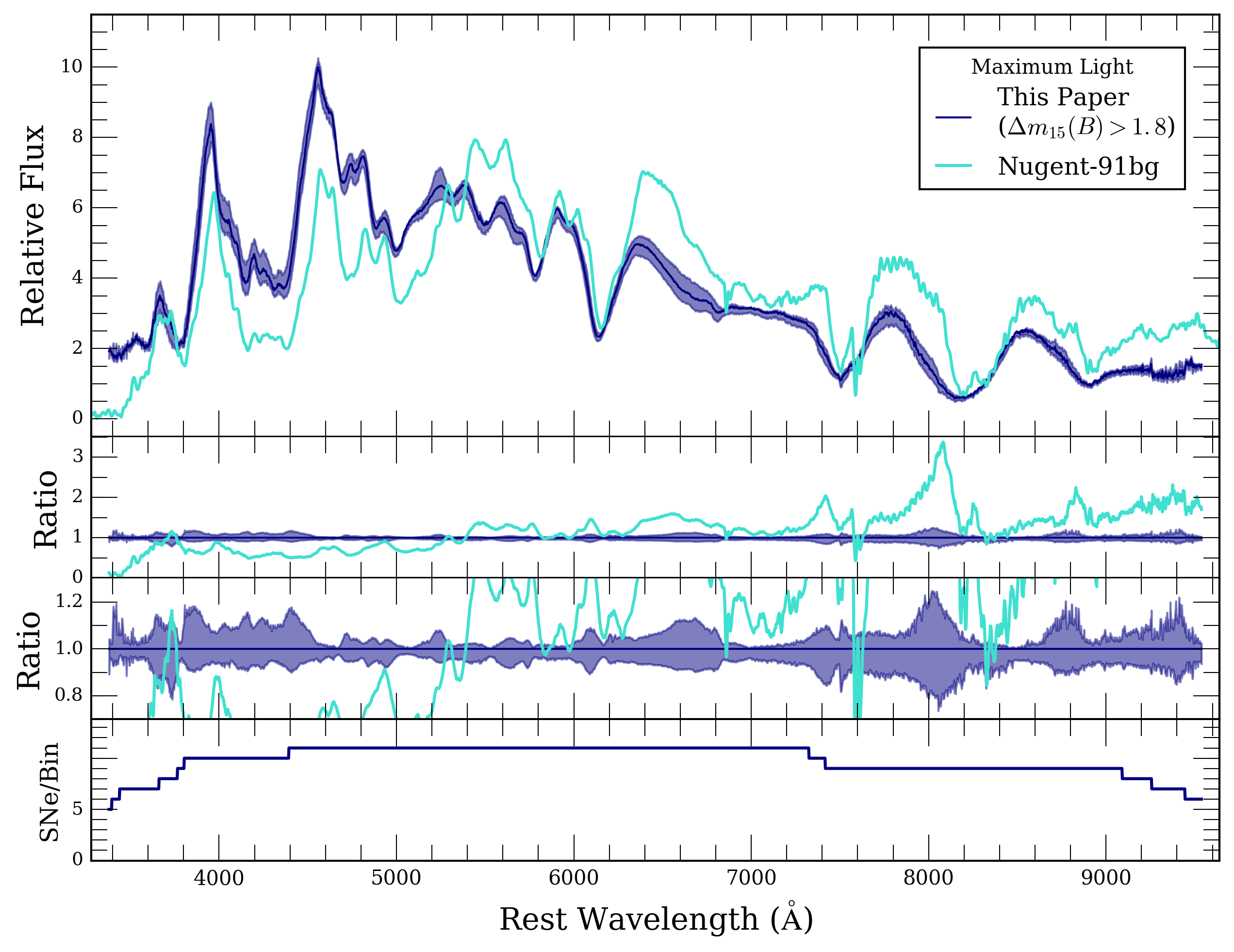siebert_template_comparisons.tar
Host-Galaxy Morphology	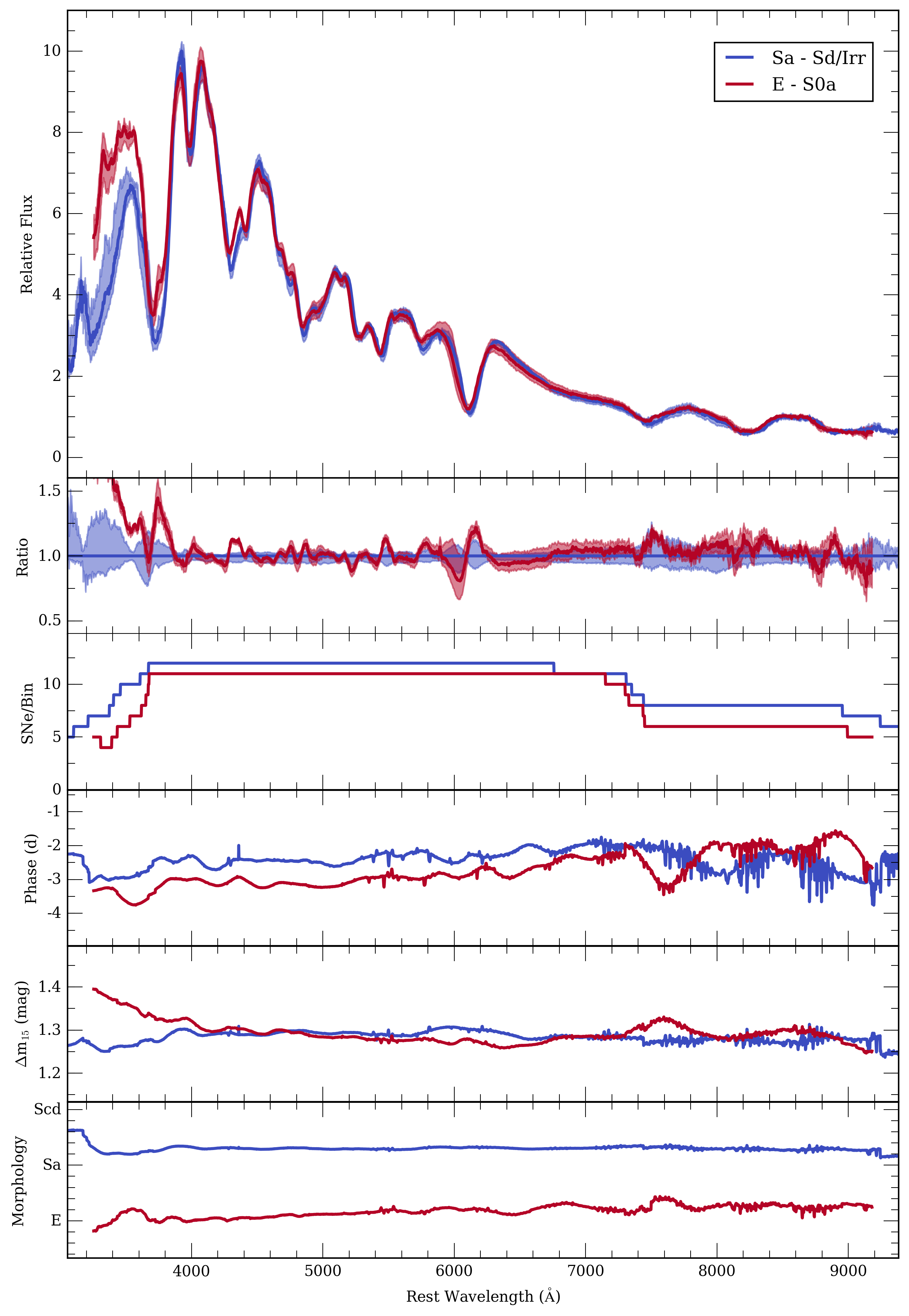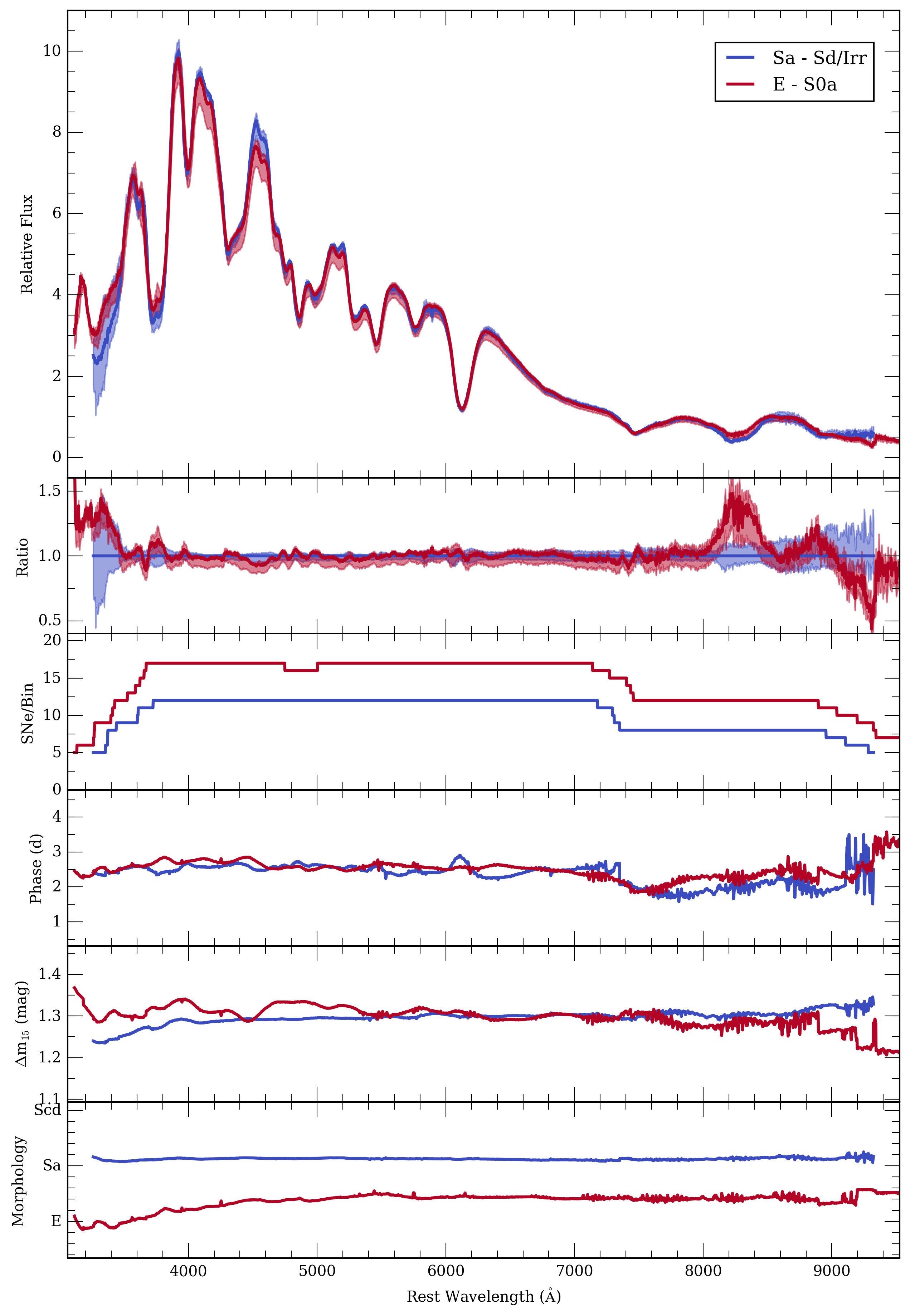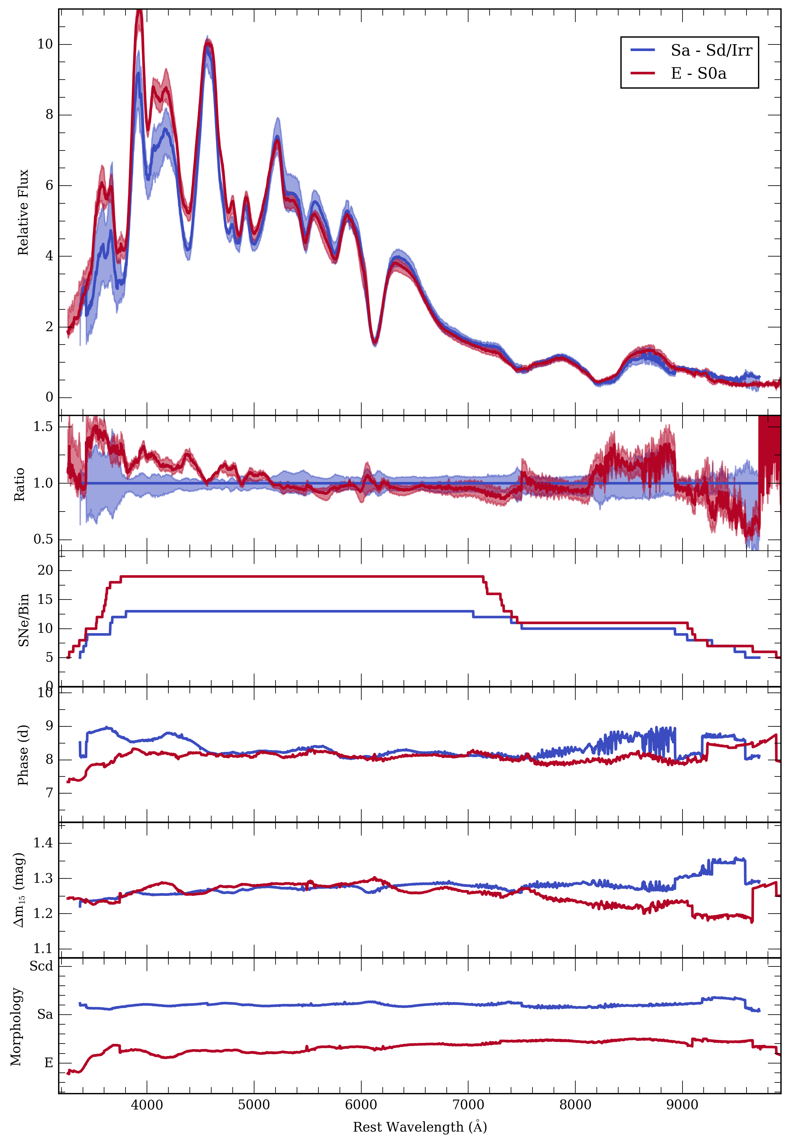siebert_host.tar